The part of this percolation argument that kept tripping me up was the collection of boxes. There is a seed box, a buffer around a different box, an auxiliary cube, a target inside a neighboring coarse box, and then a sequence of contractions and translations. What is actually moving? Why would making a target smaller help? And if fully open seeds are rare, aren’t we spending all our probability before we get anywhere?
This is the version I wanted to read: the whole geometric and probabilistic route, in pictures, with the error budgets left out. We will take the gluing theorem as given. Its matrix and cone proof is a separate project; the question here is what that theorem lets us build.
The source is OpenAI’s September 2026 preprint Critical bond and site percolation on the cubic lattice. This post explains its proposed argument, specializing to independent bond percolation in three dimensions. My animated tour discusses a related manuscript and spends more time on gluing itself.
There is also a 14-page picture guide to download. The figures below are schematic: flat squares usually stand for three-dimensional boxes, and their relative sizes are exaggerated for readability.
The route through the proof
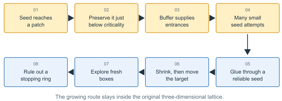
The local work makes one extension reliable. The global work makes those extensions usable repeatedly.
Open full-size diagram ↗In bond percolation, each lattice edge is independently open or closed. A cluster consists of vertices joined by open paths. Below the critical density, there is no infinite cluster; above it, there is one. The question is what happens exactly at the critical density.
The argument starts by assuming that an infinite cluster exists there. It turns this assumption into very reliable finite crossing events. Once the required boxes are fixed, lowering the edge density slightly changes those crossing probabilities only slightly. The proof then uses the surviving local crossings to construct an infinite cluster below criticality. That gives the contradiction.
The important word is finite. We are not moving the infinite-cluster event below criticality by continuity. We move a finite collection of local estimates, and build infinite growth afterward.
1. A seed catches a piece of infinity
A seed is a small cube compared with the regions we will eventually work in. It can nevertheless be very large in lattice units.
Under the contradiction assumption, an infinite cluster exists almost surely. As a centered seed box grows, it becomes increasingly likely to touch one. It does not contain the whole infinite cluster. It contains a vertex whose open paths continue outside every finite surrounding box.
That gives a reliable connection from the seed to the boundary of a larger cube. But a connection to somewhere on the boundary is too vague for the geometry ahead. We will want it to land on a particular patch.
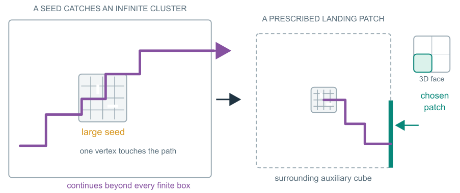
The large seed supplies a reliable way out. Symmetry and FKG turn boundary reachability into a crossing to a prescribed quarter-face.
Open full-size diagram ↗Divide each face of the surrounding cube into four quarters. Symmetry makes the probabilities of missing the different quarter-faces equal. For independent edges, these miss events are positively correlated: learning that one patch was missed can only increase the chance of missing another. The FKG inequality turns this observation into a bound on missing all the patches together. If missing the entire boundary is extremely unlikely, no prescribed quarter-face can have a large miss probability.
So we obtain a useful local statement: the seed is very likely to connect to whichever quarter-face the construction specifies in advance. We are not observing the configuration and choosing a patch it happened to reach.
At this point, the seed’s internal edges do not have to be fully open. Full opening has a different job later.
After fixing all the finite boxes needed in the construction, we lower the edge density slightly. The required local crossing tests remain reliable. Everything that follows then runs at that lower density.
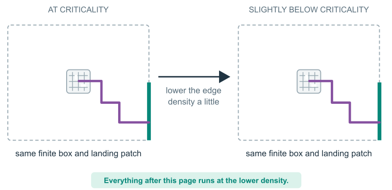
The crossing probabilities remain high. The matching purple routes are schematic; continuity does not preserve the same realized path.
Open full-size diagram ↗2. Keep the regions straight
Here is a single extension, before worrying about a whole lattice of boxes.
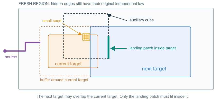
The small seed, the auxiliary cube, and the next target have different jobs. The auxiliary cube may protrude beyond the target; its selected landing patch must fit inside it.
Open full-size diagram ↗- The current target is the rectangle the incoming connection is trying to reach.
- Its buffer supplies a surrounding region with many candidate entry layers.
- A small seed is a possible attachment point near a reachable entrance.
- An auxiliary cube around that seed supplies the reliable seed-to-quarter-face crossing.
- The next target contains the selected quarter-face.
The auxiliary cubes all fit inside a larger fresh region. Fresh means that, given what has been revealed so far, its edges still have their original independent law. It does not mean that the region contains no open paths.
The extension statement controls the event that the source reaches the current target but misses the next one. This distinction matters. We have not first revealed a successful arrival and then assumed that all onward probabilities survived that conditioning.
3. The buffer supplies entrances
Picture the buffer as nested fences around the current target. If the source reaches the target, it must get through every surrounding fence.
For one candidate layer, expose the exterior connections and count the reachable entrances. If there are only a few, closing their crossing edges can seal the layer at a definite probability cost. Those crossing edges are still fresh.
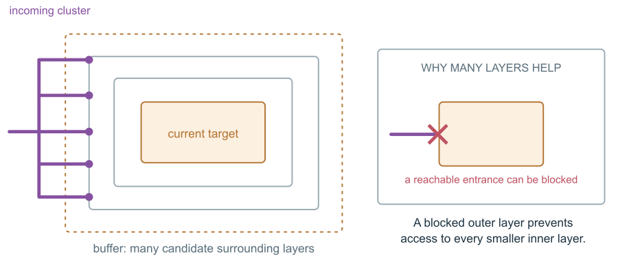
A reachable, completely sealed outer layer prevents the source from reaching a smaller inner layer. Those blocking events cannot pile up in the same configuration.
Open full-size diagram ↗Now use the nesting. Once an outer layer is reachable and completely sealed, no inner layer can also be reachable from the source. The corresponding blocking events are mutually exclusive, so their probabilities share a limited total budget.
With enough candidate layers, at least one fixed layer makes reaching the target with only a few entrances unlikely. This is the Grimmett–Marstrand layer-selection trick.
The choice is deterministic. We choose the layer from its probability estimate, before seeing which random configuration occurs. We are not searching a realized configuration for its luckiest fence.
4. Rare open seeds become useful through repetition
Near the reachable entrances, place separated seed boxes. A successful trial requires the entrance edge and all internal seed edges to be open.
That can be extremely rare. We pay for it with space: keep the seed size fixed, then arrange enough separated trials that some succeed. Each trial uses a disjoint set of fresh edges.
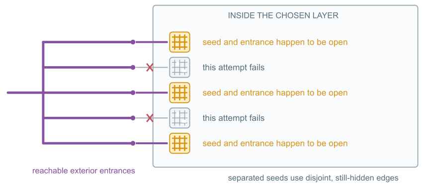
We only need some attempts to succeed. These are naturally occurring open seeds in one configuration, not edges we force open or repeatedly resample.
Open full-size diagram ↗Why insist on full opening? The local crossing estimate says that some vertex of the seed connects onward. The incoming path might attach at a different vertex. Opening every internal edge joins the incoming entrance to whichever vertex has the onward connection.
Why not use the entire buffer as one giant seed? Because increasing its size would make the all-open event rarer while leaving us with essentially one attempt. Small seeds let us increase the number of opportunities without increasing the cost of each opportunity.
There is one more filter: an attached seed should have good conditional onward prospects after the relevant interior configuration is fixed. Here, the interior means the region inside the chosen buffer layer, not just an individual seed. The proof shows that open-but-poor seeds are uncommon. The intuition is an averaging argument. Open seeds have very low average onward failure, so a large fraction of them cannot have substantial conditional failure. Many successful trials then leave a reached seed with reliable onward prospects.
5. Gluing handles the selection problem
The tempting argument is: choose the first seed the source reaches, then use that seed’s ordinary onward connection probability.
The trouble is the word first. It tells us both that one seed was reached and that earlier seeds were not. Those negative facts can reveal obstructions in the same configuration we want to use for the onward connection. An ordinary, unconditioned crossing estimate need not survive that selection.
The gluing theorem supplies the statement we need: if every relay in a specified set has reliable onward prospects, reaching the relay set but missing the target is unlikely. It handles the fact that the incoming cluster chooses its own point of attachment.
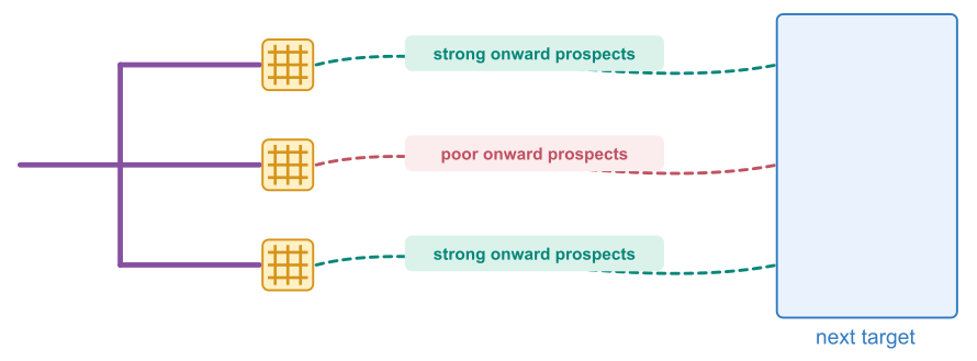
Dashed curves represent conditional prospects, not paths already revealed. Gluing handles which reliable seed the incoming connection reaches.
Open full-size diagram ↗The proof is careful about which information defines the reliable relay set. Quality is determined from the interior edges alone. Exterior information is used to locate and count incoming seed opportunities, then averaged out before applying gluing. Once only the interior is fixed, the remaining edges again have a product law and the relay-quality estimates are the right ones.
That completes one extension: many entrances, many seed trials, a reached reliable seed, then gluing to the next target.
6. Why a quarter-face fits when a full face does not
An entrance can appear near a side or corner of the allowed region. The auxiliary cube centered near that entrance may stick out above or beside the next target. Its full forward face can therefore be too large to fit.
In a two-dimensional picture, choose the half of the forward edge that points toward the target’s center. In three dimensions there are two sideways directions, so choose the inward half in each. Their combination is a quarter-face.
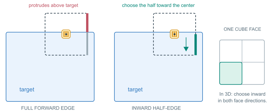
The cube can stick out of the target while its chosen landing patch stays inside. Full-cube containment in fresh space is a separate check.
Open full-size diagram ↗The normal direction, which places the face forward or inward, is checked separately. The inward choices control the two sideways coordinates. The patch can cross the target’s centerline; what matters is that it cannot escape through the opposite side under the construction’s size choices.
This is the geometric point worth retaining: the landing region has to work wherever the useful seed appears. We cannot assume a convenient central entrance.
7. Contract first, then translate
Each coarse box has a standard inner target. We want to transfer a connection from one inner target to the next.
Every use of the extension rule needs a buffer around its current target. During translation, the next target must accommodate landing patches from that expanded region. Consequently, the intermediate targets grow a little at each move. Starting at full size would leave us with a target too large to fit inside the neighbor’s standard inner box.
The construction creates room first: three contractions, one per spatial direction.
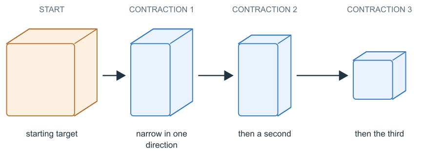
Only the targets change. The centers stay fixed during contraction; the shapes are separated here for comparison. Small buffer allowances are omitted.
Open full-size diagram ↗Contraction does not preserve connectivity automatically. The source could reach the large target and miss the smaller one. We use the same extension lemma to make that outcome unlikely, aiming a suitable quarter-face inward so that it lands in the smaller central region.
Nothing is cut out of the open cluster. We ask for an additional connection to a smaller target. Paths are undirected: they may turn toward the center before continuing toward the neighboring box.
After those three contractions come ten translations. There is no contraction between the ten moves. The target shifts toward the neighbor and grows slightly to absorb the buffers, using the room created at the start.
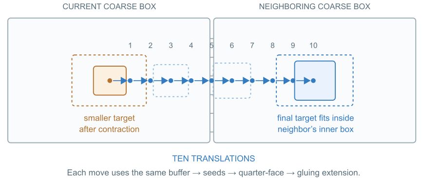
One coarse box-to-box crossing uses all thirteen steps. The final target fits inside the neighbor’s standard inner target, so the construction can be repeated.
Open full-size diagram ↗Three reflects the spatial directions. Ten reflects the chosen box separation and step length. Thirteen is their total. The proof needs a fixed finite number of valid moves; these particular counts are not claimed to be minimal.
The moves are event comparisons in the same configuration, not independent trials along a prescribed route. If the source reaches the first target but misses the last, some neighboring pair of targets is where the extension failed. That lets the local failure bounds control the whole crossing.
8. Explore without consuming tomorrow’s information
We now have a reliable neighboring-box connection estimate. Using it repeatedly requires more care than simply declaring boxes independently good.
A good box adds unvisited neighbors to a queue and becomes their parent. Following the parents back to the root gives a parent chain. A queued box carries a strong prediction that the source connects to its inner target through that chain. All earlier boxes on the chain have been processed. The only remaining unknown edges relevant to the prediction lie in the pending box and its incoming parent interface.
Reserve those edges until the box’s turn. Processing other boxes cannot touch them. The prediction therefore stays valid while the box waits.
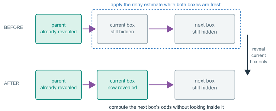
The relay estimate is applied before revealing the current box. Afterward, compute the next box’s connection prospects without inspecting its actual edges.
Open full-size diagram ↗When a pending box is processed, reveal its interior and incoming interface. This decides whether its own connection succeeded. For each unvisited neighbor, calculate the chance of extending the connection into that neighbor, averaging over its still-hidden edges.
Calculating a probability does not reveal an outcome. The queue, parent assignments, and good/bad decisions are functions of already observed edges and these calculations. They add no hidden information about the remaining edge values.
A box is good only if its own connection is verified and its unvisited neighbors have strong connection predictions. A bad box produces no children. The relay estimate shows that a processed box is unlikely to be bad, conditional on the entire prior history.
The exploration starts on a positive-probability event where the root box and its outgoing interfaces are open. That finite initialization cost is paid once. The subsequent steps have to remain reliable throughout the growing exploration.
9. Why the boxes form a two-dimensional grid
The coarse boxes are arranged on a square grid. Each still contains a three-dimensional piece of the original lattice: its internal paths can move in all three directions.
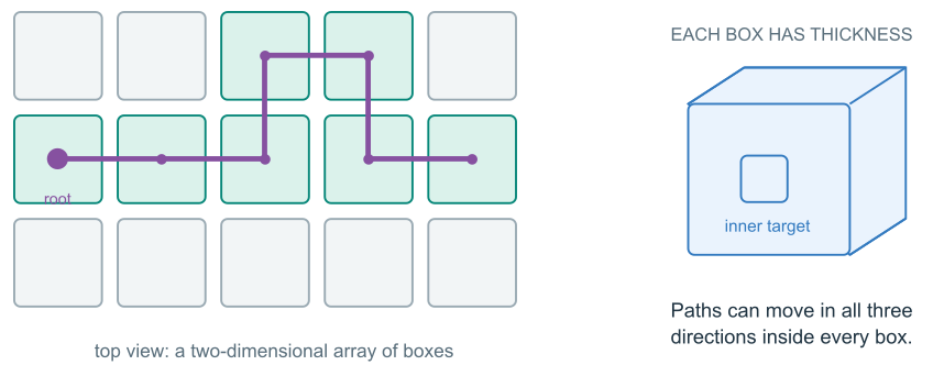
The array is two-dimensional; the paths inside its boxes are three-dimensional. An infinite route through this thick planar array is sufficient.
Open full-size diagram ↗This is closely related to the Grimmett–Marstrand slab architecture. A slab is infinite in two directions and bounded in the third. A planar array of uniformly thick boxes lives in such a slab, and an infinite cluster there is also an infinite cluster in the full lattice.
The planar arrangement gives a convenient description of how growth could stop. If the good cluster is finite and the queue empties, every outside neighbor of that cluster has been processed and declared bad. Its boundary contains a surrounding dual loop.
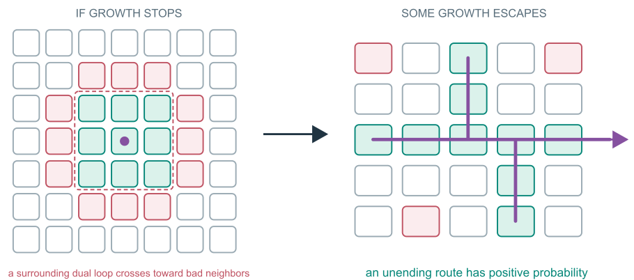
Stopping every route requires a surrounding obstruction. Counting possible loops and controlling collections of bad boxes leaves a positive chance that the exploration never stops.
Open full-size diagram ↗Individual steps being reliable would not, by itself, guarantee success along an infinite prescribed chain. The grid offers alternative routes. The contour argument controls the collective obstruction needed to stop them all.
It does not assume that the good/bad classifications are independent. The conditional bound from the exploration is strong enough to control the probability that any specified collection of boxes is processed and declared bad. That is the input used in the loop count.
With positive probability, infinitely many boxes are good. Each has a verified connection back to the original source, so the source belongs to an actual infinite open cluster. All of this is happening at the slightly lowered density. The contradiction is complete.
10. What gluing changes about the older argument
Grimmett and Marstrand proved that supercritical percolation survives inside a sufficiently thick slab. Their method already had open seeds, geometric steering, and sequential exploration. It also confronted the problem that an explored cluster has a revealed closed boundary.
They crossed that boundary using sprinkling: a small increase in openness. Many boundary locations have useful onward routes, and the added openness gives chances to activate a connection through one of them. Their original paper uses site percolation; in the bond picture, think of adding extra open edges.
That expense is affordable for a supercritical result. Start above criticality, but below the desired final density, and reserve the remaining margin for the extra openings. Their construction keeps the accumulated increases controlled. See Grimmett–Marstrand, Lemma 6 and Section 4.
For the critical-point argument, spending extra density would lose the desired contradiction: an infinite cluster above criticality is expected. Kozma and Nitzan identify precisely this obstruction in their reduction to a gluing inequality.
Here, gluing supplies the extension bound at the current density. Once the finite estimates have been moved slightly below criticality, the construction can continue without adding openness.
What I want to remember
The important distinctions are about information and geometry:
- A seed likely to touch an infinite cluster is not the same condition as a seed whose internal edges are all open.
- Reaching a fixed target set is not the same as conditioning on the first relay reached.
- A region can contain open paths and still be fresh, because its edge values have not been learned.
- Contraction changes what we ask the cluster to reach. It does not delete or squeeze the cluster.
- A two-dimensional array of boxes can carry fully three-dimensional paths.
The numerical margins make these operations compatible. The ideas explain why the operations exist at all. When I return to the matrix and cone proof, the question it has to answer is now quite concrete: how can an incoming connection use a reliable onward route when its choice of relay is biased by the same random configuration?
Sources and related reading
- Critical bond and site percolation on the cubic lattice, OpenAI, September 24, 2026. The manuscript followed here, pinned to the cited repository revision. Sections 3–6 contain the finite crossings, extension lemma, neighboring-box geometry, and exploration.
- A reduction of the θ(p_c) = 0 problem to a conjectured inequality, Gady Kozma and Shahaf Nitzan, 2024. The gluing problem and the finite-to-infinite reduction framework.
- The supercritical phase of percolation is well behaved, Geoffrey Grimmett and John Marstrand, 1990. Seeds, nested layers, sprinkling, and dynamic renormalization.
- Animated tour and a closer look at gluing.
- Download the illustrated picture guide.